Understand your Event Segmentation analysis
An Event Segmentation analysis shows how often actors perform events and how those results differ across groups of actors. Each module in the template controls one part of the question the analysis answers. The template consists of the following modules:
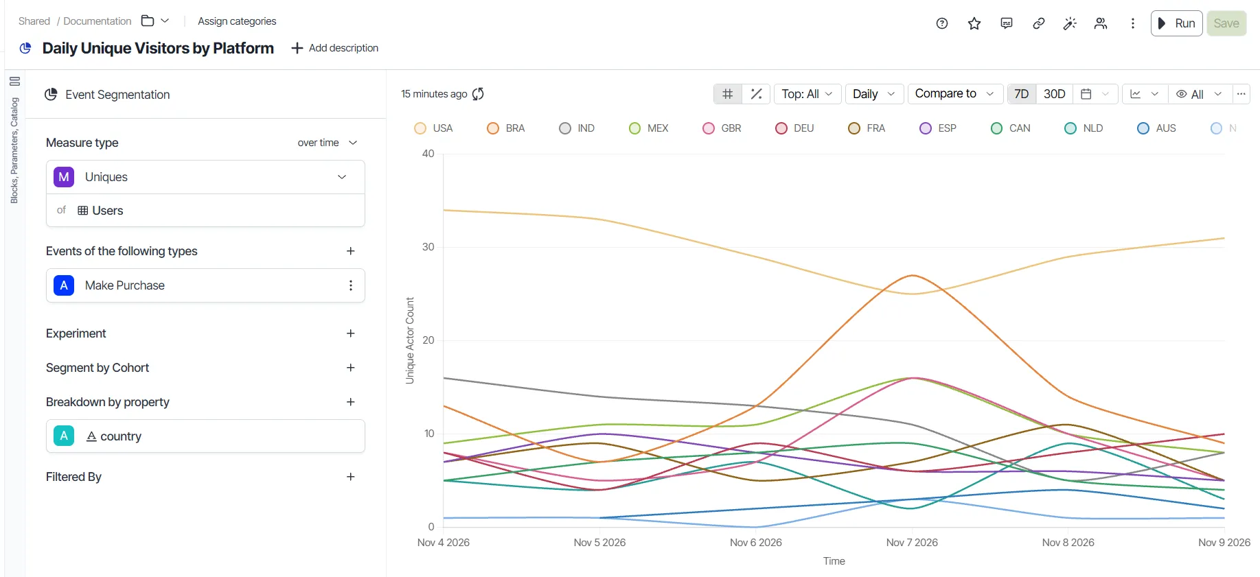
Measure module
Choose the measure that the analysis calculates for the selected events and segments. The measure decides what the chart reports, such as the total number of events or the number of distinct actors.
An Event Segmentation analysis measures the following:
- Count of Events – The count of events during a specified time frame.
- Uniques – The count of unique users triggering events.
- Frequency – The distribution of actors by the number of times they performed an event.
- Average Events – The average number of events performed by an actor.
- Intervals Engaged – The count of time buckets for each actor, in which that actor met the engaged event criteria.
- Active % – The count of users who performed any active event.
- Aggregate by Property – Custom aggregate for actors who did at least one of the events.
- Metric – A metric from the catalog or a custom block.
To see a measure change over time, click the not over time drop-down list and choose Over time. Results over time let you set up period-over-period comparison for each measure.
A metric is a custom measure derived from the same event dataset that the analysis uses, like ProductInteractions. The metric aggregates data from that dataset.
For example, a Freemium to Enterprise Ratio metric divides Freemium user events by Enterprise user events. In an Event Segmentation analysis, this metric shows a typical ratio of four to six freemium events per enterprise event. For Add Data Source events, the ratio drops to one to two. The lower ratio indicates that enterprise users rely on that feature more than freemium users.
The Uniques, Frequency, Intervals Engaged, Active %, and Average Events measures count actors instead of events. These measures add a catalog picker where you choose the actor to count, such as Users. The Active % measure requires an active event annotation on your event stream.
Create a custom measure over multiple event streams
Create a custom measure when the prebuilt measures in Analytics do not answer your question. A custom measure combines events from more than one event stream in a single formula. Add a formula block, and then choose it as the measure in the Measure module.
The following example calculates the number of purchases for each user who viewed a product details page (PDP).
- Go to + > Event Segmentation.
- Choose Make Purchase for event A.
- Choose View PDP (Product Details Page) for event B.
- In the block shelf, click + > Formula to create a formula block.
- Enter count(@A) / uniques(@B.user_id) as the formula. In this formula, count(@A) is the number of purchases, and uniques(@B.user_id) is the number of unique users who viewed a PDP.
- Click Apply.
- Choose Metric or Block in the Measure module.
- Choose the formula block as the value.
- (Optional) Choose country in the Breakdown by property section to compare the results by country.
- Click Run.
- Click Save.
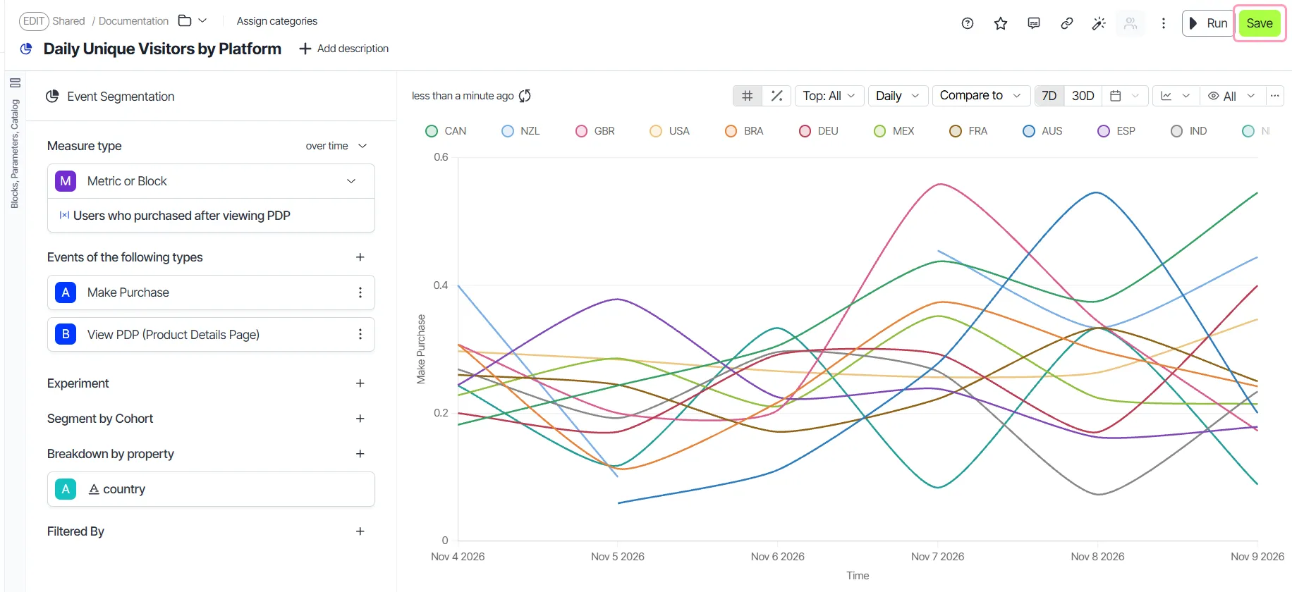
Events module
Choose one or more events to analyze. The events you choose define the behavior that the analysis measures.
The event picker displays event streams and their event types. In Analytics, event streams are datasets configured to model event flows. Not every dataset is an event stream. For example, the Users dataset lists users instead of events.
Hover over an event to see its usage stats, including the average events received per day. Use the stats to judge whether an event still receives data. See Event taxonomy.
Note
When the platform has a single dataset, the event selector shows only event types. It hides the event streams selector and lists event types in a drop-down list. The selector also includes a filter for choosing events based on conditions. When you choose a JavaScript Object Notation (JSON) column, it expands to show the available keys. Choose a key and click Apply to use the path of that key as the column display name.
Choose which event occurrences to count
Choose which occurrences of an event count toward the Uniques measure to separate new behavior from repeat behavior. For example, count only users who played content for the first time ever. The chart then shows new adopters instead of returning users.
Each event in the Events module has its own occurrence setting. The setting is available only when the measure is Uniques.
- Choose Uniques in the Measure module.
- Hover over an event in the Events module.
- Click All events in time range.
- Choose one of the following options:
- All events in time range – Counts each actor who performed the event at any point in the selected time range. This option is the default.
- First event in time range – Counts only the first occurrence of the event by each actor within the time range. Occurrences before the time range do not affect the count.
- First event ever – Counts an actor only when their first-ever occurrence of the event falls within the time range. The count excludes actors who performed the event before the time range.
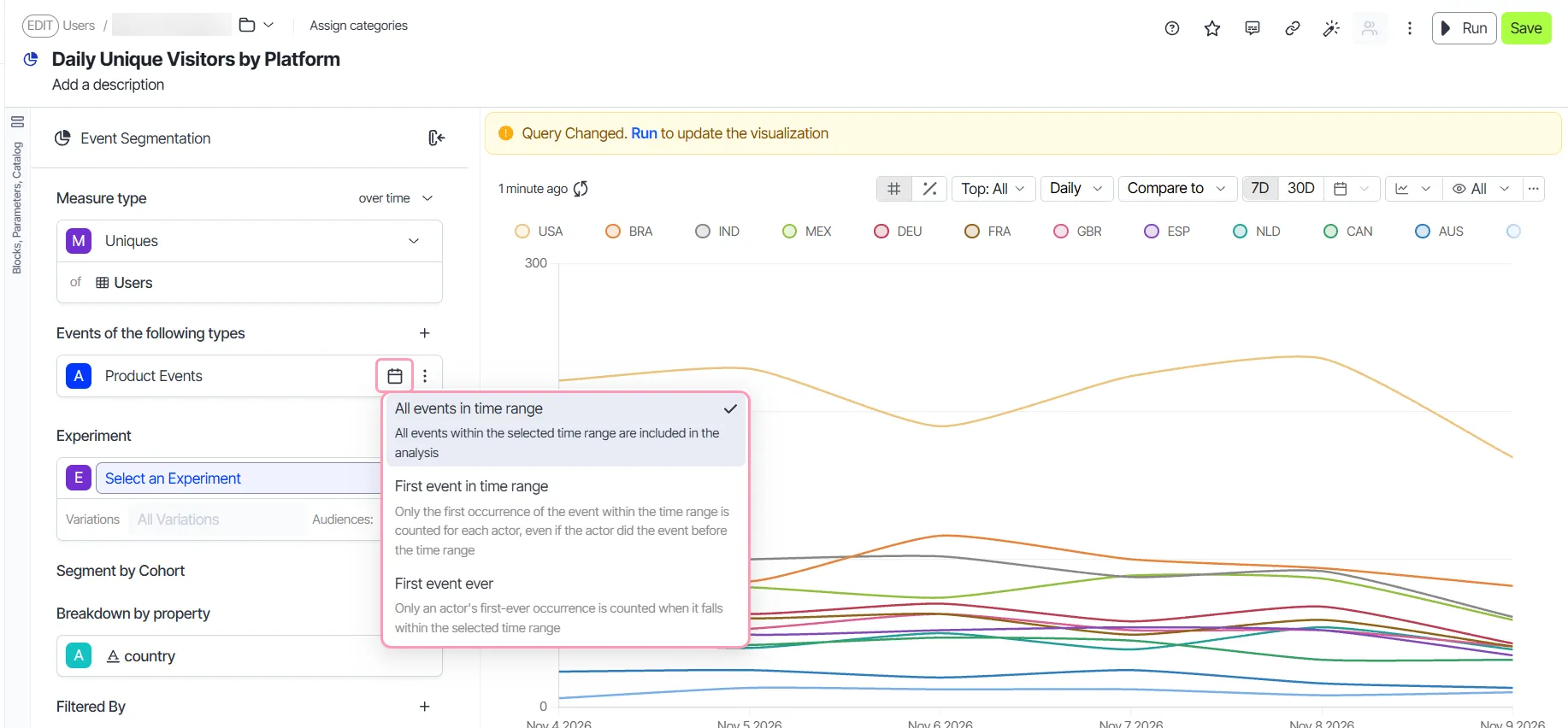
- Click Run to update the analysis.
A non-default option displays its name as a label on the event. The label tells readers that the analysis does not count every occurrence. Click the label to change the option.
Segmentation module
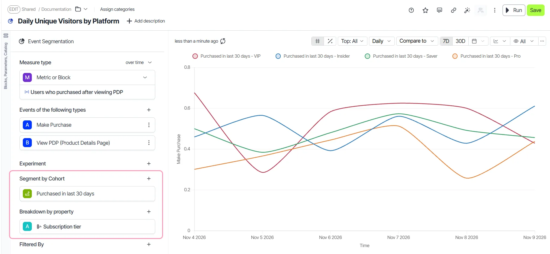
Compare groups of actors, such as users, to see how the measure differs between them. Add cohorts in the Segment by Cohort section. Add properties in the Breakdown by property section. Choose an existing cohort from the drop-down list. To define a behavioral cohort block in one click, click New Cohort.
Filters module
Narrow the data in a visualization to answer a more specific question. For example, define a region filter to see results for one region only.
The Filters module also lets you choose JSON columns. When you click a JSON column, it expands to display its keys. Choose a key and click Apply. The selected key becomes the display name for that column.
Visualization module
Present the analysis results in the format that best answers your question. In this module, edit the visualization, examine the underlying Structured Query Language (SQL) query, and add charts to a dashboard.
Six visualization types are available: Line Chart, Bar Chart, Pie Chart, Horizontal Bar Chart, Single Value, and Table. A Pie Chart shows the distribution of events by segmentation attribute across the selected time range.
The following features are available in this module:
- # and % – Switch between numbers and percentage values on your chart.
- Top 'N' segments – Choose the number of top segments to display in the visualization.
- Time range and time grain – Configure the time range and time grain of the analysis.
- Sampling – Configure sampling and responses for the analysis.
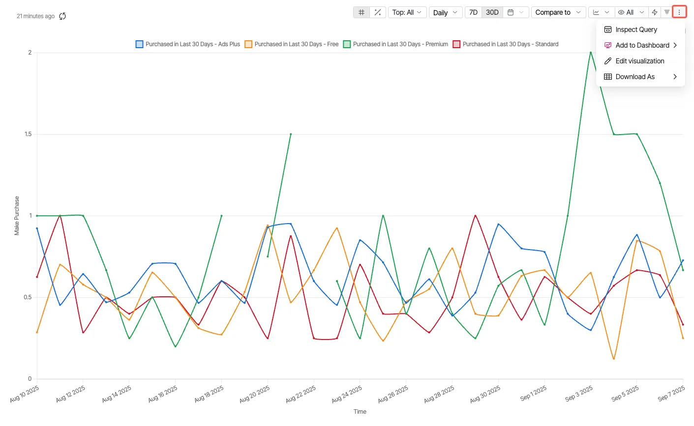
- Edit visualization (Other actions) – Inspect queries, edit visualizations, add analyses to dashboards, and download comma-separated values (CSV) files.
Switch between numbers and percentages
Switch the y-axis between absolute numbers and percentages in one click to compare segments of different sizes. Absolute numbers give a clearer breakdown of how many actors are in each segment. Click # for numbers or % for percentages.
Top N segments
Limit the chart to the segments with the most activity so the visualization stays readable. Click the Top drop-down list, choose or enter a number, and click Apply. The total count of selected events decides which attribute values rank highest. Beelines also let you set the number of top segments.
Time range and time grain section
Configure the time range and time grain to control which events the analysis includes and how it groups them. The time range is the complete period of events that the analysis includes. For example, use the last two years or the dates between two specific days. The time grain is the granularity of the analysis, such as Daily (one day) or Weekly (seven days).
Set the time range from the drop-down list, or choose a quick option. Try different time ranges and time grains without leaving the chart. To set a lag, click Offset, and then set Ending.
Choose a sampling mode
Choose a sampling mode to balance query speed against result precision. Click the sampling control in the visualization toolbar. Its tooltip shows the current sampling mode. The Sampling Mode drop-down list offers three modes: Disabled, Enabled - Faster Response, and Enabled - Higher Precision.
Series-level customization
Keep a series in the same color across charts so that dashboards are easier to read. Override the default color and display name for individual data series from the chart legend. See Override the palette for an exploration.
Edit visualization section
- Inspect Query – Click this option to open a query inspector. It has three tabs, SQL, Warehouse SQL, and NetScript. You can change the SQL and NetScript queries by clicking the Open as SQL Explore and Open as NetScript Explore buttons in the respective sections.
- Add to Dashboard – Add the exploration you created to a dashboard. You can choose from two options: Pick a dashboard or New Dashboard.
- Edit visualization – Edit the chart settings. It has two sub-sections: Visualization and Sorting.
- Under Visualization, you can configure
- Automatic refresh for your chart.
- Chart type.
- X-axis and Y-axis configuration.
- Tooltip.
- Size configuration.
- Under Sorting, you can
- Enable the sorting option on the graph.
- Configure sorting rules and the limit.
- Download As - Download your analysis in either CSV or EXCEL format. The system preserves the column formatting for the downloaded files as well.
Note
A pie chart that segments by several cohorts counts an event or actor one time per cohort that contains it. A pie chart shows a whole divided into non-overlapping parts, so overlapping cohorts inflate the total.