Frequentist (Fixed Horizon) statistics
Products
- Optimizely Feature Experimentation
- Optimizely Analytics
Feature availability depends on your plan type. For questions, contact your Customer Success Manager.
Fixed Horizon is a frequentist statistical method for traditional A/B tests with a predetermined sample size. Use it when you want to evaluate results one time, after the experiment collects enough data for a reliable conclusion. The method relies on established statistical concepts such as p-values, minimum detectable effect (MDE), and variance. These concepts determine whether the differences you observe between variations are meaningful. The following sections explain each element and how it affects experiment design and analysis.
To configure a Frequentist (Fixed Horizon) test in Feature Experimentation, see Configure a Frequentist (Fixed Horizon) A/B test.
Why Frequentist (Fixed Horizon) tests require a predetermined sample size
Calculate the sample size before you start a Frequentist (Fixed Horizon) experiment so you can trust its result. A predetermined sample size gives you the following benefits:
- Reliable conclusions – You collect enough data to detect a real effect instead of missing it in the noise.
- No mid-test peeks – You avoid the extra false positives that early looks at partial data cause.
- A clear decision rule – You evaluate results one time, against thresholds you set in advance.
Important
Viewing or acting on incomplete results increases false positives and invalidates your experiment.
Sample size calculation
Know which inputs drive the sample size so you can plan how much traffic your experiment needs. The required sample size per variation depends on the following inputs:
- Baseline metric value – The current performance of the metric you are testing.
- MDE – The smallest relative change you want to detect.
- Statistical significance level – Your confidence threshold.
- Variance – The spread of your metric values.
These inputs together determine the number of visitors each variation needs for a reliable conclusion. To compute that number, use the Frequentist (Fixed Horizon) Sample Size Calculator.
How visitors count toward the sample size
Understand which visitors count toward the sample size so you can estimate how long your experiment needs to run.
The sample size is a lifetime total for each variation. Optimizely does not reset it daily or weekly. Optimizely counts each visitor once, when the visitor first sees a variation. The experiment reaches its sample size when every variation reaches the target.
Your experiment configuration in Optimizely Experimentation determines which visitors count. For example:
- Desktop-only targeting – Only desktop visitors count toward the sample size.
- Mobile-only targeting – Only mobile visitors count toward the sample size.
- No platform targeting – Every visitor who qualifies for the experiment counts, on any platform.
Breaking down results by a segment, such as desktop and mobile, does not change the required sample size. A breakdown only changes how you view the results. Optimizely checks the combined visitors in each variation against the sample size, not the visitors in each segment.
The date range and filters of an Experiment Scorecard limit which visitors count. Visitors outside the date range or excluded by a filter do not count toward the sample size.
Why early looks at results cause false positives
Wait for the full sample before you act on results so that random chance does not decide your experiment. In a Fixed Horizon experiment, every early look at results raises the chance of a false positive. An early look tempts you to stop the experiment before it collects the full sample. You then believe you found a winner when random chance caused the effect.
For example, suppose you flip a coin 100 times to test whether it is fair. After 10 flips, you see seven heads and risk wrongly concluding that the coin is unfair. Waiting for all 100 flips gives a more reliable answer.
Fixed Horizon example scenario
Follow this example to see how calculator inputs become a sample size and minimum duration. The example also shows what those numbers mean while the experiment runs.
Example inputs
The example uses the following Sample Size Calculator inputs:
- Baseline Metric Value – 5%
- Minimum Detectable Effect – 10% relative increase. You expect the metric value in the treatment to be 5\% \times (100 + 10)\% = 5.5\%.
- Statistical Significance Level – 95%
- Number of Variations – Two (one baseline and one treatment)
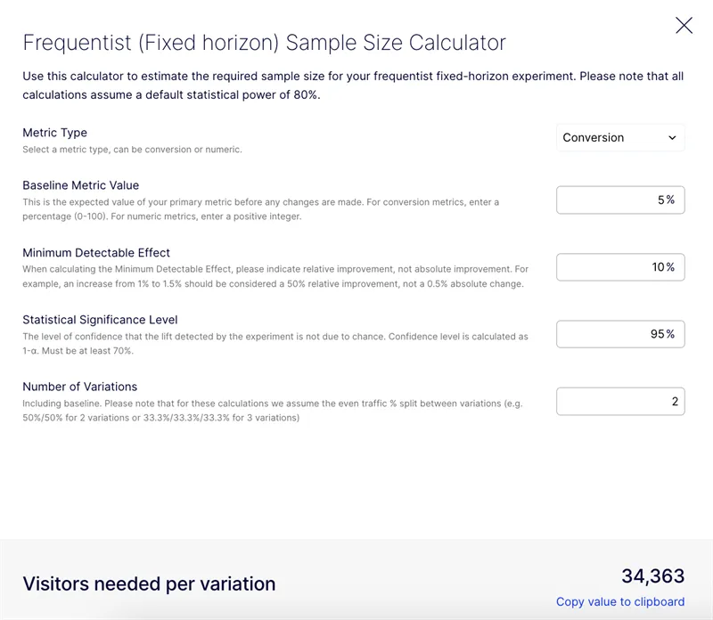
Calculated sample size and duration
The example produces the following requirements:
- Visitors needed per variation – 34,363 visitors
- Minimum duration – Seven days
Run every test for at least one business cycle (seven days) to account for changes in user behavior. For example, visitors often behave differently on weekends than on weekdays. See Seasonality and traffic spikes.
What the requirements mean for your experiment
The requirements set when you can act on the results:
- Run the experiment until each variation receives 34,363 visitors and at least seven days pass.
- Until the experiment meets these conditions, the results show visitors and improvement for each variation. Statistical significance and confidence intervals display only after the experiment meets them.
Statistical calculations
The formulas in the following sections show how Optimizely calculates Fixed Horizon results, so you can reproduce or audit them. The formulas assume two variations:
- One baseline (control) group
- One treatment (test) group
With multiple treatments, Optimizely compares each treatment group to the baseline group, which creates a series of two-sample comparisons. Each extra comparison raises the chance of a false positive. This multiple comparison problem requires false discovery rate control.
Confidence interval calculations
A confidence interval gives the range of improvement values that fit your data at your chosen significance level. Use it to judge how precise an observed improvement is. Optimizely picks the calculation based on the metric type (binary, numeric, or ratio) and the improvement type (absolute or relative). The following section covers numeric and binary metrics with relative improvement.
Numeric or binary metric, relative improvement
The calculation uses the following definitions:
- Let \hat{\theta}_h and \hat{\sigma}^2_h denote the estimated metric (sample mean) and variance in the baseline (control) group with sample size n_h.
- Let \hat{\theta}_t and \hat{\sigma}^2_t denote the estimated metric and variance in the treatment group with sample size n_t.
- Let \hat{R} := \frac{\hat{\theta}_t}{\hat{\theta}_h}. The relative improvement is 100(\hat{R} - 1)\%.
The Delta method gives the following approximate 100(1 - \alpha)\% confidence interval:
\hat{R} - 1 \pm \Phi^{-1}(1 - \alpha/2)\sqrt{\frac{1}{\hat{\theta}_h^2} \left( \frac{\hat{\sigma}_h^2 \hat{R}^2}{n_h} + \frac{\hat{\sigma}_t^2}{n_t} \right)}Because Optimizely reports and tests relative improvement, the previous confidence interval is a Wald interval. To test absolute improvement, consider a t-test instead.
P-values
A p-value is the probability of a result at least as extreme as yours if the variations do not differ. When the p-value is smaller than one minus your significance level (0.05 for a 95% level), the difference is statistically significant. Each Wald confidence interval has a corresponding p-value.
Let w denote the observed value of the Wald statistic W. Calculate the p-value with the following formula:
p\text{-value} = \mathcal{P}_{\theta_0}(|W| > |w|) \approx 2\Phi(-|w|)Sample size estimation calculations
Estimate how many visitors an experiment needs to detect a given improvement at your chosen power and significance level. Power is the probability that the experiment detects a real effect of the size you expect.
Estimation for relative improvement for binary or numeric metrics
Use this formula to estimate the baseline group sample size before you start an experiment. Suppose the true ratio of treatment to control is \gamma and n_t = kn_h. The following formula gives the sample size that achieves the power 1 - \beta:
n_h = \frac{\frac{1}{\theta_h^2} \left( \sigma_h^2 \gamma^2 + \frac{\sigma_t^2}{k} \right)} {\left(\frac{1 - \gamma}{z_{\alpha / 2} + z_\beta}\right)^2}Calculate metric variance
The sample size formula needs the variance of your metric (\sigma_h^2 and \sigma_t^2). Calculate the variance from historical data with a variance function or by hand.
If you store per-visitor values for the metric (for example, revenue per visitor), use one of the following variance functions:
- Excel or Google Sheets – =VAR.S(A2:A1000)
- Structured Query Language (SQL) – SELECT VAR_SAMP(METRIC_VALUE) FROM YOUR_EVENTS
Most analytics and business intelligence tools include a sample variance function.
To calculate the variance by hand, follow this example. Suppose your last five visitors spent $10, $20, $30, $40, and $50:
- Find the average. The average is $30.
- Subtract the average from each value. The results are −20, −10, 0, 10, and 20.
- Square each result:
- (−20)² = 400
- (−10)² = 100
- 0² = 0
- 10² = 100
- 20² = 400
- Add the squared results: 400 + 100 + 0 + 100 + 400 = 1000.
- Divide the total by the number of values minus one: 1000 ÷ (5 − 1) = 250. Divide by the number of values minus one because the data is a sample, not the full population.
The variance is 250.
Next steps
See the following articles for related information: